Introduction to the optimization method of differential amplifier performance

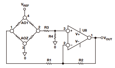
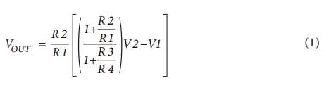
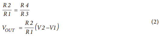
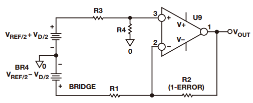
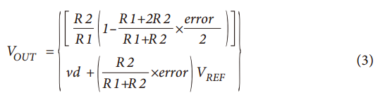
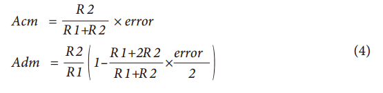
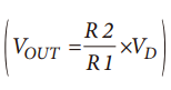
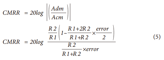
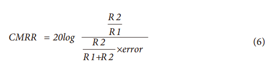
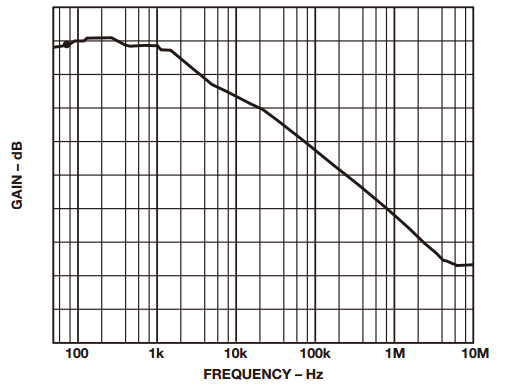
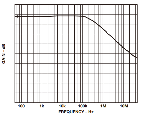
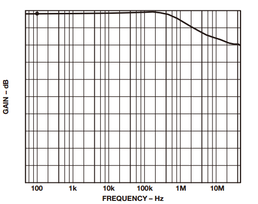
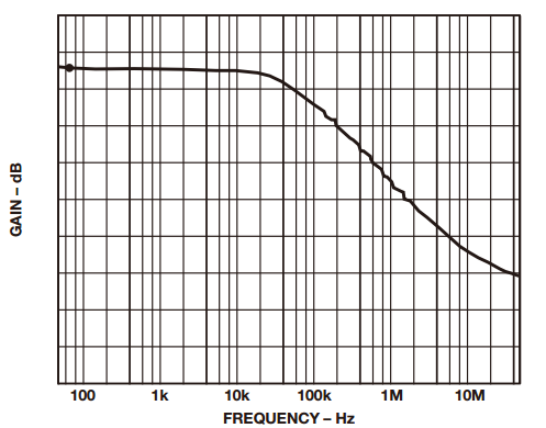
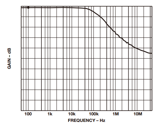
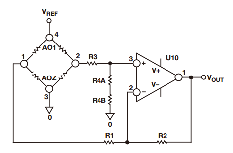
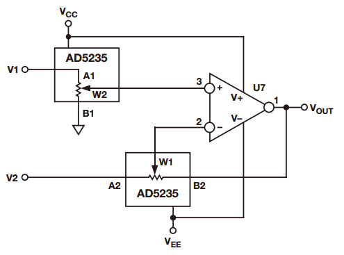
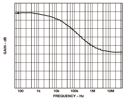
Sometimes it is necessary to measure small signals with large common mode signals.

In this type of application, an integrated instrumentation amplifier with two or three operational amplifiers is typically used. Despite the excellent common mode rejection ratio (CMRR) of instrumentation amplifiers, price factors and performance metrics hinder their use in such applications.

Let's share the construction of the differential amplifier and its performance optimization method!

The instrumentation amplifier may not have the bandwidth, DC accuracy, or power consumption required by the user. Thus, in this case, the user can build a differential amplifier with a single amplifier and an external resistor instead of the instrumentation amplifier. However, unless a well-matched resistor is used, the common-mode rejection ratio of this circuit will be poor. This application note explores several ways to build discrete differential amplifiers and optimize their performance. It also recommends several op amp products that make the overall cost-effectiveness of the solution comparable to monolithic instrumentation amplifiers.

Figure 1 shows the use of a typical differential amplifier constructed from a single amplifier that is connected to a sensor bridge.

figure 1

According to the superposition principle, the output of the circuit is a function of the difference between the two inputs. The transfer function of the circuit shown in Figure 1 is:

A special case occurs in the following situations:

Equation (1) can be simplified to equation (2):

The output is equal to the difference between the two inputs multiplied by the gain factor, which can be set to 1. Equation 2 holds when the resistance ratio matches well. Assume that the perfect match resistance values ​​are: R2 = R4 = 10 kΩ, R1 = R3 = 1 kΩ, V1 = 2.5 V, V2 = 2.6 V, then VOUT = 1 V.

As described above, one of the disadvantages of the circuit shown in Fig. 1 is that its common mode rejection is relatively low due to resistance matching errors. For the sake of discussion and clarity, we redraw the circuit diagram, as shown in Figure 2.

figure 2

The error caused by the tolerance of resistor R2 is R2 (1 – error). By superposing the principle, while making R1 = R3, R2 = R4, after calculating and arranging, the output voltage (VOUT) is:

According to Equation 3, the common mode gain (Acm) and the differential gain (Adm) can be defined as:

It can be seen from Equation 4 that when there is no error in the resistance value (ie, error = 0), then Acm = 0, and the amplifier responds only to the differential voltage, then:

Therefore, when the resistance ratio error is zero (error = 0), the common-mode rejection ratio of the circuit will depend to a large extent on the common-mode rejection ratio of the selected amplifier. When the resistance ratio error is not zero, as shown in Figure 2, the circuit common mode rejection ratio can be expressed as:

When the R2 error is extremely small, the second term in the above equation is negligible and:

For a unity-gain discrete differential amplifier with R2 = R4 = 10 kΩ, R1 = R3 = 10 kΩ and error = 1%, the common-mode rejection ratio is approximately 46 dB. This is much worse than the performance of a monolithic differential amplifier (AMP03), which is shown in Figure 3.

Figure 3. AMP03 (monolithic differential amplifier) ​​common-mode rejection ratio versus frequency

As indicated above, errors due to resistor mismatch can constitute a major disadvantage of discrete differential amplifiers. But there are ways to optimize this circuit.

➤ a. In Equation 3, the differential gain is proportional to the ratio of (R2/R1). Therefore, one way to optimize the performance of the above circuit is to place the amplifier in a high gain configuration as much as possible (using a large resistor in a high gain setting can cause noise problems, which also needs to be addressed).

By selecting R2 and R4 (R2 = R4) with larger resistance values, and R1 and R3 (R1 = R3) with smaller resistance values, higher gain can be obtained, so that the common mode rejection ratio is better. For example, when R2 = R4 = 10 kΩ, R1 = R3 = 1 kΩ, and error = 0.1%, the common mode rejection ratio will be improved, better than 80 dB. For high gain configurations, choose an IB very low, very high gain amplifier (such as the AD8551 family of amplifiers from Analog Devices) to reduce gain error. The gain error and linearity of the circuit are a function of amplifier performance.

Figure 4a. Common mode rejection ratio of AD8605 (where G = 1)

Figure 4b. Common mode rejection ratio of the AD8605 (where G = 10)

➤ b. Select a resistor with a smaller tolerance and higher accuracy. The more the resistance is matched, the better the common mode rejection ratio. For example, if the above circuit requires a common mode rejection ratio of 90 dB, the resistance matching tolerance should be around 0.02. In this case, the common-mode rejection ratio of the circuit is no less than that of some high-precision instrumentation amplifiers, but their AC and DC characteristics are better.

Figure 5a. Common mode rejection ratio of OP1177 (where G = 1)

Figure 5b. Common mode rejection ratio of OP1177 (where G=10)

➤ c. Another way to improve the common mode rejection ratio of the circuit shown in Figure 1 is to use a mechanical trimming potentiometer, as shown in Figure 6.

Figure 6

With this method, the user can use a lower tolerance resistor, but it needs to be adjusted periodically.

➤ d. As an alternative to circuits where accuracy is not critical, a digital potentiometer can be used, as shown in Figure 7. The AD5235 (a non-volatile memory, dual 1024-bit digital potentiometer) with the AD8628 forms a differential amplifier with a gain of 15 (G = 15).

By using a potentiometer, you can gain programming power and complete gain settings and fine-tuning in one step. Another advantage of this circuit is that the dual resistor (AD5235) has a temperature coefficient of 50 ppm, making it easier to match the resistor ratio. Other digital potentiometers are also available depending on the accuracy and tolerances required for the circuit.

Figure 7

Figure 8. Common mode rejection ratio and frequency of the circuit shown in Figure 7.

➤ e. Use a dual or quad amplifier to build an instrumentation amplifier with better common-mode rejection ratio and higher input impedance. This is a more costly solution and a method used by monolithic instrumentation amplifiers. The corresponding amplifiers should be selected according to actual needs, such as better BW, ISY and VOS. Such requirements may not be met by instrumentation amplifiers.

Auto-zero amplifiers such as the AD8628 and AD855x families are the best choice for this type of application. These amplifiers have extremely high dc accuracy and do not add any error to the output. The auto-zero amplifier has long-term stability and does not require repeated calibrations like some systems. The minimum common-mode rejection ratio of the auto-zero amplifier is 140 dB, so resistor matching will be the limiting factor in most circuits. Therefore, it is best for users to build a differential amplifier and optimize its performance according to the above guidelines.