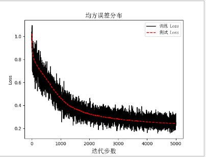
This time, I use TensorFlow to write a neural network. This neural network is very simple to write. On three layers, the input layer--hidden layer----output layer; First import the package we want to use # -*- coding: utf-8 -*-import tensorflow as tfimport matplotlib.pyplot as pltimport numpy as npimport matplotlibfrom sklearn import datasetsfrom matplotlib.font_manager import FontProperties Then, when setting up our drawing, we should display the Chinese font, because Python comes with an explanation that does not support Chinese. #设置ä¸æ–‡font = FontProperties(fname=r"c:\windows\fonts\simsun.ttc", size=14)zhfont1 = matplotlib.font_manager.FontProperties(fname=r'c:\windows\fonts\simsun.ttc' ) Define a session because the diagram must be started in the session # Define a graph session sess=tf.Session() Here I use the data set of the public data Iris, although this data set is played by everyone, but this is a learning code, it does not care so much; #莺花花数æ®é›†iris=datasets.load_iris()x_vals=np.array([x[0:3] for x in iris.data])y_vals=np.array([x[3] for x in iris.data ]) Set a random seed here, in order to let everyone reproduce the results. #Set a seed to find the result seed=211tf.set_random_seed(seed)8np.random.seed(seed) Beginning with a well-defined data set, one is the training set, one is the test set, the training set accounts for 80%, and the test set accounts for 20%. # 分测试机 and training set train_indices=np.random.choice(len(x_vals),round(len(x_vals)*0.8), replace=True)test_indices=np.array(list(set(range(len(x_vals) ))-set(train_indices)))x_vals_train=x_vals[train_indices]x_vals_test = x_vals[test_indices]y_vals_train = y_vals[train_indices]y_vals_test = y_vals[test_indices] Here we are normalizing the features, that is, converting all numerical features to values ​​between 0-1, using the feature maximum distance as the denominator; there are other standardization methods that are of interest to understand. The advantage is that it can make iterations faster, and it is to eliminate the dimension, which is the impact between units; The function nan_to_num is mainly used to eliminate the computational impact of the None value. #Normalization function def normalize_cols(m): col_max = m.max(axis=0) col_min = m.min(axis=0) return (m - col_min) / (col_max - col_min)#Data normalization and transfer Empty set x_vals_train=np.nan_to_num(normalize_cols(x_vals_train))x_vals_test=np.nan_to_num(normalize_cols(x_vals_test)) Ok, the above has generated the data set we want; here we set the data set for training once, generally choose 2^N multiple, because the computer is binary storage, so fast, here I choose A 25, because the data set is relatively small, no effect Batch_size=25 Define the training variables Y and X here, and set them as floating point types by the way. X_data=tf.placeholder(shape=[None,3],dtype=tf.float32)y_target=tf.placeholder(shape=[None,1],dtype=tf.float32) Here we set the number of hidden layer connections #设置Hide layer hidden_layer_nodes=5 Start defining the parameter variables for each layer because the input variables are three # Define each layer variable, the initial variable is 3 A1=tf.Variable(tf.random_normal(shape=[3,hidden_layer_nodes]))b1=tf.Variable(tf.random_normal(shape=[hidden_layer_nodes]))A2=tf .Variable(tf.random_normal(shape=[hidden_layer_nodes,1]))b2=tf.Variable(tf.random_normal(shape=[1])) Here we use the relu function as the activation function, and the output also uses the relu function. # Define the output of the hidden layer and the output of the output layer hidden_output=tf.nn.relu(tf.add(tf.matmul(x_data,A1),b1))final_output = tf.nn.relu(tf.add(tf.matmul (hidden_output, A2), b2)) Here we are defining the loss function, which is useful for maximum likelihood estimation. Here we use the mean square error method. Loss=tf.reduce_mean(tf.square(y_target-final_output)) Define the update method and learning rate of the parameters. Here we use the gradient descent method to update. The next time we explain the update in other ways, and the learning rate decreases with the number of iterations, tfboys is so capricious. #declare algorithm initial variable opt=tf.train.GradientDescentOptimizer(0.005)train_step=opt.minimize(loss)# variable to initialize init=tf.initialize_all_variables()sess.run(init) Define two lists to store the error of the test set and training set in training #è®ç»ƒè¿‡ç¨‹loss_vec=[]test_loss=[] Start the iteration, here we set the number of iterations to 5000 For i in range(5000): #Select the dataset of batch_size size rand_index=np.random.choice(len(x_vals_train),size=batch_size) #Choose the data set rand_x=x_vals_train[rand_index] rand_y=np.transpose([ Y_vals_train[rand_index]]) #Start the training step sess.run(train_step,feed_dict={x_data:rand_x,y_target:rand_y}) #Save the loss result temp_loss=sess.run(loss,feed_dict={x_data:rand_x,y_target:rand_y }) #Save loss function loss_vec.append(np.sqrt(temp_loss)) test_temp_loss = sess.run(loss, feed_dict={x_data: x_vals_test, y_target: np.transpose([y_vals_test])}) test_loss.append(np. Sqrt(test_temp_loss)) #print loss function, print once 50 times if (i+1)%50==0: print('Generation: ' + str(i + 1) + '. Train_Loss = ' + str( Temp_loss)+ '. test_Loss = ' + str(test_temp_loss)) The final result of the iteration is Next, we look at the trend of error changes with iteration, the decline is not fast enough, the code is still very rough, too many places need to be optimized; next time I am writing an optimized version #画图plt.plot(loss_vec, '', label='trainingLoss') plt.plot(test_loss, 'r--', label='testLoss') plt.title('mean square error distribution', fontproperties= Font)plt.xlabel('iteration step', fontproperties=font)plt.ylabel('Loss')plt.legend(prop=zhfont1)plt.show() Special Wire Rope For Port And Engineering Machinery special wire rope, wire rope for port machinery, wire rope for engineering machinery ROYAL RANGE INTERNATIONAL TRADING CO., LTD , https://www.royalrangelgs.com
(2)")